Approximations of the posterior in Gaussian process regression

Gaussian process (GP) regression scales cubically in , the number of regression points. As a result, approximations of the posterior distribution are of interest. This note describes five approximations:

• Subset of data,
• Subset of regressors,
• Fully independent training conditional,
• Randomised Nyström.

I originally wrote these notes for a student, but I thought they would make for a nice blog post as well!

Preliminaries

Suppose we have a multivariate Gaussian partitioned into two vectors , . The joint distribution with marginal mean and covariances is given by

where

for some covariance function .

We can write the marginal distribution as

Basics of Gaussian process regression

Given a set of pairs of training points and outputs , compute the predictive distribution of the function values at test locations . We sometimes omit dependence on when it’s obvious.

The assumptions for GP regression are:

• Gaussian observations: ‘s are related to via additive noise :
• Gaussian function evaluations: function values are distributed according to Our goal is to compute the posterior predictive distribution . Let’s first compute the joint Gaussian:

since it’s easy to go from a joint to a conditional via a Schur complement. The mean of is zero by assumption, so that’s easy. By assumption, the likelihood is and we therefore have

Since , what’s left to do is to compute the off-diagonals of the covariance:

In summary,

Using what we know about conditional Gaussians, the posterior is just

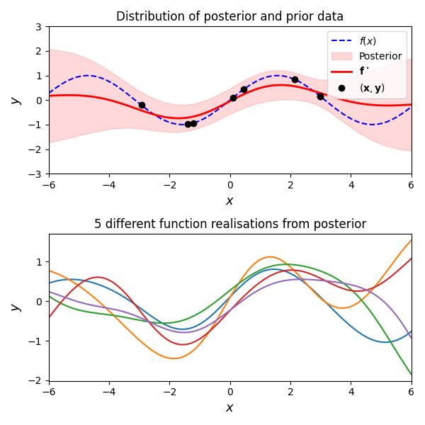
Draws from the predictive distribution

Let’s look at a concrete example of a GP and and a few draws.

Inducing points approximations

The full predictive distribution requires the inversion of a matrix. To reduce the computational burden of GP regression, let us introduce a set of inducing points, or inducing variables:

Now the conditional independence approximation is the following:

that is,

Let us explore how affects the posterior.

Subset of data (SD)

We simply select of the data points for training, where is small enough that is acceptable from a computational point of view. This is the most crude approximation.

Subset of regressors (SoR)

First, we note that , so

which means

The SoR approximation is simply to take this quantity as deterministic, i.e.,

The SoR covariance function is therefore

This can be seen by evaluating

We can use the covariance function to compute and By replacing with gives us the posterior:

We can rewrite this as follows using the Sherman-Morrison-Woodbury identity:

where

Fully Independent Training Conditional (FITC)

This is a fairly simple extension of SoR, at least from a linear algebra point of view. Recall

from which

While the SoR approximation causes the posterior covariance matrix to degenerate by the assumption that

FITC is basically a compromise between a degenerate (zero) covariance and the full covariance above. Indeed, FITC just takes the diagonal:

Like before, we combine this with our prior and obtain

Randomised Nyström

Let be a matrix with random Gaussian entries. The randomised Nyström approximation of the kernel matrix is where . As a result,

References

• Quinonero-Candela, Joaquin, and Carl Edward Rasmussen. “A unifying view of sparse approximate Gaussian process regression.” Journal of machine learning research 6.Dec (2005): 1939-1959.
• Halko, Nathan, Per-Gunnar Martinsson, and Joel A. Tropp. “Finding structure with randomness: Probabilistic algorithms for constructing approximate matrix decompositions.” SIAM review 53.2 (2011): 217-288.